✓ Legenda of Formulas
CALCULATING NUMBER OF BUSINESS DAYS
To calculate business days, start with a specific date and count the number of working days excluding weekends and public holidays. Various online tools and software applications are available to simplify this process, allowing you to input the start and end dates and receive the accurate count of business days in between.
Distinguishing between business days and calendar days is crucial. Calendar days include all days in a week, including weekends and public holidays. On the other hand, business days focus solely on the working days when regular business operations take place. The differentiation between the two is vital when setting deadlines, planning projects, or estimating delivery times.
In financial analysis, to calculate the number of Business Days is useful to measure the time length associated to a specific indicator which is relevant to assess the relative strength intensity.
For example, when you measure the difference between the quotes and the moving average of a specific equity (stock or index) you may assess the period of time the moving average is above or below the market quotes.
The same is for other indicators and their moving averages (RSI, volumes).
CAGR - COMPOUNDED ANNUAL GROWTH RATE
How to Calculate Compound Annual Growth Rate (CAGR)
The Compound Average Growth Rate (CAGR) is the rate of interest accrued (i.e., earned) on not only the original investment but also on any previously accrued interest from a prior period. It is typically used to measure an investment’s historical rate of return, allowing the investor to forecast future returns.
There are many ways to calculate the CAGR, such as with the calculator above, the CAGR formula, a spreadsheet, or a financial calculator. All you need to know is the beginning and ending amount and the time period in years.
CAGR Formulas
This first CAGR formula can only be used for annual compounding. The CAGR formula for other compounding periods is explained later in this section.
CAGR Formula with Annual Compounding
The formula to calculate CAGR with annual compounding is:

N = number of years
1/N = the N power root of the ratio between the Endings Value and the Starting Value.
Thus, the compound annual growth rate is equal to the ending value EV divided by the beginning value BV to the power of 1 divided by the number of years n, minus 1.
Simple vs. Compound Annual Growth Rate
The simple annual growth rate (SAGR) differs from the compound annual growth rate in that the growth is only calculated on the beginning value.
In the DJI example, the SAGR will need to be higher to achieve the same ending value because the SAGR does not include compounding.
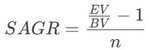
BV = beginning value
EV = ending value
n = number of years
What is the Compound Annual Growth Rate Used For?
The Compound Annual Growth Rate is primarily used by investors to analyze how well an investment or portfolio has performed over a particular time period. Investors are then able to compare their performance to a particular benchmark.[2]
For instance, an investor might choose to compare the growth of an investment to the Dow Jones Industrial Average as their benchmark. If their portfolio’s CAGR consistently outperforms this benchmark, they are investing better than the market. They are underperforming if their CAGR is consistently lower.
It is important for investors to choose a benchmark that is comparable to their portfolio, to get a like-for-like comparison.
For example, if an investor is investing primarily in bonds, then a benchmark composed of stocks is not going to provide useful results. Also, if an investor is invested in stable value stocks, the NASDAQ, which is composed of technology and growth stocks, won’t provide useful results either.
Why is CAGR Important?
As discussed in the previous section, the CAGR gives investors useful information regarding stock performance by calculating the CAGR on their portfolio and comparing it to similar benchmarks.
If a stock has been underperforming every year, the investor may decide to cut their losses and remove it from the portfolio in favor of another which has been overperforming.
Or, if their portfolio has been underperforming the benchmark for a while, they may decide to switch up their strategy entirely and outsource the stock-picking to mutual funds or exchange-traded funds (ETF).
On the other hand, if their portfolio is consistently beating the market, they can make the decision to reduce their risk if the market falls (risk-averse investors) or increase their risk if they believe they can continue outperforming the market (risk-seeking investors). Either way, the CAGR provides the necessary information to analyze stocks and portfolios better.
The CAGR is also important because it uses a compound rate, as opposed to a simple rate, as shown earlier. The compound rate is the true return and can therefore be compared to other forms of investments more easily.
The simple growth rate of over 16% calculated earlier is misleading. If you were to invest at the same rate of 16.55% for five years, you would have more than doubled the investment, which is not what actually happened with the DJI over this timeframe.
For example, the chart below shows an investment accruing a compound growth rate of 16.55% vs. the Dow Jones Industrial Average. You can see that a compound growth rate of 16.55% results in doubling the investment, while the simple growth rate observed with the growth of the DJI did not.
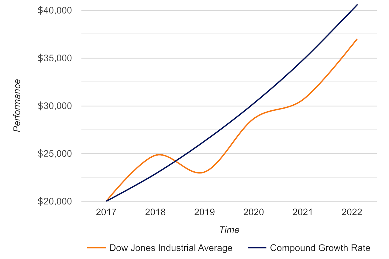
Performance of the Dow Jones Industrial Average from 2017 through 2021 compared to a similar investment with a compound annual growth rate of 16.55%.
To approximate how long it would take to double an investment, you can also use the Rule of 72. The approximate time it will take for an investment to double in value can be calculated by dividing 72 by the interest rate.
In our example, it would take roughly 4.349 years (72 ÷ 16.5544) to double an investment earning 16.55% per year using the Rule of 72. Note that the Rule of 72 should be used for quick approximations, the exact time to double at this rate is actually 4.525 years, which is calculated using a more complex formula.
Pros and Cons of Using CAGR
The two pros of using the CAGR were discussed in the previous section. First, it allows investors to make important decisions regarding their portfolios and the components of their portfolios.
Second, since it uses a compounding rate, it provides the true growth rate over the time period since it accounts for returns on accrued interest or growth, versus a simple growth rate which results in higher returns when accrued growth is factored in.
There are three cons of using CAGR:
- First, it assumes constant growth each year. For example, in the table shown above, each year the DJI increased by 12.2451%. We know this is not accurate; the graph above illustrates the volatility in performance over time. Some years, it may have increased by 20% or 30%, while some years it may have stayed flat or even declined. This is due to the risk inherent in the investment. If there was no risk, then each year it would increase by the same amount. There is no investment out there that guarantees a specific rate of return each year. The higher the risk, the higher the expected return. Other external factors (e.g. supply and demand, inflation, & other economic factors) also play a role here and contribute to the risk of an investment.
- The second con of using the CAGR is that it is unable to account for trading decisions in the portfolio. We briefly discussed this earlier. In our example, where our portfolio increased from $10,000 to $19,500, we needed to mention that there was no buying or selling during that time. If there were, it would muddy the true results and not allow us to accurately compare the portfolio to the benchmark. For example, what if $5,000 was added to the portfolio over this time? Then we could say that most of the growth was really due to just the additions to the portfolio instead of growth within the portfolio.
- Finally, CAGR does not take the amount of risk into account. If two investments had a 5-year CAGR of 10%, how would we know which one is better? The answer lies in the risk. Investors use different ways to measure risk, but the most common ones are either the standard deviation or beta. Both standard deviation and beta both measure the volatility of an investment. If there are higher swings in one stock or the other, the standard deviation and beta will also be high. Beta is a measure of volatility relative to other investments, while standard deviation is a measure of the volatility over time without regard to other investments. An investor would prefer to invest in the stock that has the lower standard deviation and beta, assuming the CAGR is the same between them.
CAGR vs. IRR
The CAGR measures the growth rate of a portfolio, whereas the Internal Rate of Return (or IRR) measures whether an investment in capital expenditure makes financial sense for a business. Both assess investments, but they are used for different purposes.
The CAGR can be used for an investment that grows over time. As has been discussed throughout, the easiest example is the stock market. You invest in a stock with the expectation that the value will increase over time.
This will give you a return of capital appreciation and dividend payments (for stocks that distribute dividends).
The CAGR needs to be compared to a benchmark in order to judge its success. For example, if your portfolio earned 15% over the prior year, that may seem like a great year. Earning 15% per year over the long run is a great return that few investors can attain.
The IRR analysis is used in capital budgeting to determine the rate of return on a project or capital expenditure. The IRR that is calculated from a stream of payments needs to be higher than the business’s IRR for it to be considered.
The IRR is the rate that sets the present value of a stream of payments to $0. With a business project or capital expenditure, there is typically an initial outflow of cash followed by a stream of inflows of cash.
The IRR that the business uses will need to be what other projects have yielded or the return that the owners demand.
Let’s set up an example for a business to see how it works. An addition of a new machine costs $10,000 upfront but provides savings of $3,000 per year for four years, at which point it will be scrapped. What is its IRR?
By using our IRR calculator, you can find that the IRR is 7.71%. The calculator discounts each cash flow by the IRR to obtain its present value. Once added to the -$10,000 initial cash flow, the total is $0.
If the company requires an IRR of 10%, then this project should not be pursued. If the required IRR is 5%, then the business should proceed with adding the new machine.
INTERNAL RATE OF RETURN (IRR) AND NET PRESENT VALUE (NPV)
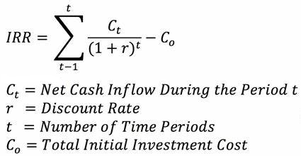
How to Calculate Internal Rate of Return
The internal rate of return (or IRR) is the rate that sets the net present value (NPV) of a stream of cash flows for a project to $0.[1]
NPV is a tool used in corporate finance to assign a dollar value to future returns on an investment. We cover NPV in more detail below, and you can also learn more about it on our NPV calculator.
The higher the IRR, the more financially successful a project is. A project’s IRR needs to be higher than the company’s required rate of return in order for the company to move forward with a project.[2]
The minimum required rate of return, sometimes referred to as the hurdle rate, is usually set at the weighted-average cost of capital (WACC) for the investment.
The IRR is essentially the compounded annual growth rate that a project is expected to earn. If a project has an initial investment of $1,000 and earns a 15% internal rate of return for five years, it is equivalent to earning 15% over five years.
While this 15% is not earned consistently each year, the IRR smooths out the return over the lifetime of the project. Try our ROI calculator to see what the compounded annual growth rate is on an investment.
The IRR assumes that each cash flow is received/paid at the end of the year. This is not a likely assumption but allows for simplicity in the calculation.
Internal Rate of Return Formula
The following formula expresses the internal rate of return. The internal rate of return is equal to the discount rate where the sum of cash flows divided by the discount rate for each time period, minus the initial investment is equal to zero.
What is the Difference Between IRR and Net Present Value (NPV)?
NPV is another tool used in corporate finance and capital budgeting to value a potential investment opportunity. It is similar to the present value but subtracts the initial investment at the end.
While the IRR is a rate of return, NPV is a dollar amount.
The NPV formula looks like this:
Note that this is similar to the formula to calculate IRR above, but in this case the NPV is not required to equal $0.
The IRR is a rate of return, but the NPV is a dollar amount. In both cases, the higher the amount, the better. They both tell the same story.
If a company calculates a negative NPV on a project, it should avoid it. It can do nothing and earn an NPV of $0, which is higher than a negative value. If the NPV comes to exactly $0, then the company will be indifferent between investing in the project and not investing in the project.
In both cases, its NPV is $0. If the project has a positive NPV, the company should move forward with the project.
The company could also use the IRR to judge potential investment opportunities. If the IRR is less than the required rate of return, then the company should not pursue the investment.
If the IRR is equal to the required rate of return, the company will be indifferent between investing or not investing. Finally, if the IRR is greater than the required rate of return, the company should invest in the project.
References
Kierulff, H., IRR: A Blind Guide, American Journal Of Business Education, July/August 2012, 5(4), 417-426. https://files.eric.ed.gov/fulltext/EJ1056227.pdf
Heisinger, K., Ben Hoyle, J., Accounting for Managers - 8.3 The Internal Rate of Return, https://2012books.lardbucket.org/books/accounting-for-managers/s12-03-the-internal-rate-of-return.html
Wendorf, M., How To Calculate Internal Rate Of Return (IRR), Seeking Alpha, July 12, 2022, https://seekingalpha.com/article/4520014-irr-formula-calculation
YIELD TO MATURITY (YTM)
What is Yield to Maturity?

Yield to Maturity (YTM) represents the total return that is generated once a bond has paid all coupon payments and reached maturity, which is when the face value of the bond will be paid to the bondholder.
In other words, YTM represents an annualized figure of what bondholders can expect to receive. Bonds, unlike stocks, do not offer speculative paybacks. The coupon payments and future value have already been determined and the only way for the bond issuer to not pay them is to default.
YTM calculations typically include a few basic assumptions. Namely, that the bond will be paid as promised (i.e., there is no default) and the bond will be held until maturity. YTM is also sometimes referred to as a bond’s redemption yield.
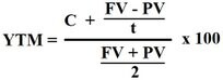
Yield to Maturity Formula
Graphic showing the yield to maturity formula where the ytm is equal to C plus the FV minus the PV divided by n, divided by the FV plus the PV divided by 2.
In order to calculate the YTM for a coupon-issuing bond, you must know the coupon rate, the bond’s face value, the present value (which should equal the current price), and the number of years to maturity.
With most bonds, this information should be clearly evident on the bond itself. But if you don’t have the physical bond in front of you, you can easily find this information within any bond-holding account.
You can use the following formula to calculate a bond’s yield to maturity:
C = coupon rate
FV = face value
PV = present value (current price)
n = years to maturity
FIBONACCI WAVES (EXTENSIONS AND RETRACEMENTS)
What Are Fibonacci Waves (Extensions and Retracements) ?
Fibonacci waves are a tool that traders can use to establish profit targets or estimate how far a price may travel after a pullback is finished. Waves levels are also possible areas where the price may reverse.
Drawn as connections to points on a chart, these levels are based on Fibonacci ratios (as percentages). Common Fibonacci extension levels are 61.8%, 100%, 161.8%, 200%, and 261.8%.1
Creating Fibonacci Extensions
Fibonacci extensions don't have a formula. When the indicator is applied to a chart, the trader chooses three points. The first point chosen is the start of a move, the second point is the end of a move and the third point is the end of the retracement against that move. The extensions then help project where the price could go next. Once the three points are chosen, the lines are drawn at percentages of that move.
Extensions are drawn on a chart, marking price levels of possible importance. These levels are based on Fibonacci ratios (as percentages) and the size of the price move the indicator is being applied to.
How to Calculate Fibonacci Retracement Levels
You can calculate Fibonacci retracement levels by completing the following steps:
Multiply the difference between points one and two by any of the ratios desired, such as 1.618 or 0.618. This gives you a dollar amount.
If projecting a price move higher, add the dollar amount above to the price at point three. If projecting a price move lower, subtract the dollar amount from step one from the price at point three.1
For example, if the price moves from $10 to $20, back to $15, $10 could be point one, $20 point two, and $15 point three. The Fibonacci levels will then be projected out above $15, providing levels to the upside of where the price could go next. If instead, the price drops, the indicator would need to be redrawn to accommodate the lower price at point three.
If the price rises from $10 to $20, and these two price levels are points one and two used on the indicator, then the 61.8% level will be $6.18 (0.618 x $10) above the price chosen for point three. In this case, point three is $15, so the 61.8% extension level is $21.18 ($15 + $6.18). The 100% level is $10 above point three for an extension level of $25 ((1.0 x $10) + 15).
The ratios themselves are based on something called the golden mean or ratio.3 To learn about this ratio, start a sequence of numbers with zero and one, and then add the prior two numbers to end up with a number string like this: 0, 1, 1, 2, 3, 5, 8, 13, 21, 34, 55, 89, 144, 233, 377, 610, 987...
The Fibonacci extension levels are derived from this number string. Excluding the first few numbers, as the sequence gets going, if you divide one number by the prior number, you get a ratio approaching 1.618, such as dividing 233 by 144. Divide a number by two places to the left and the ratio approaches 2.618. Divide a number by three to the left and the ratio is 4.236.
The key Fibonacci extension levels include 23.6%, 38.2%, 50%, 61.8%, and 78.6%.45 Also common are 100%, 161.8%, 200%, and 261.8%.5 The 100% and 200% levels are not official Fibonacci numbers, but they are useful since they project a similar move (or a multiple of that move) to what just happened on the price chart.
What Do Fibonacci Extensions Tell You?
Fibonacci extensions are a way to establish price targets or find projected areas of support or resistance when the price is moving into an area where other methods of finding support or resistance are not applicable or evident.
If the price moves through one extension level, it may continue moving toward the next. That said, Fibonacci extensions are areas of possible interest. The price may not stop or reverse right at the level, but the area around it may be important. For example, the price may move just past the 1.618 level, or pull up just shy of it, before changing directions.
If a trader is long on a stock and a new high occurs, the trader can use the Fibonacci extension levels for an idea of where the stock may go. The same is true for a trader who is short. Fibonacci extension levels can be calculated to give the trader ideas on profit target placement. The trader then has the option to decide whether to cover the position at that level.
The Difference Between Fibonacci Extensions and Fibonacci Retracements
While extensions show where the price will go following a retracement, Fibonacci retracement levels indicate how deep a retracement could be. In other words, Fibonacci retracements measure the pullbacks within a trend, while Fibonacci extensions measure the impulse waves in the direction of the trend.
Limitations of Using Fibonacci Extensions
Fibonacci extensions are not meant to be the sole determinant of whether to buy or sell a stock. Investors should use extensions along with other indicators or patterns when looking to determine one or multiple price targets. Candlestick patterns and price action are especially informative when trying to determine whether a stock is likely to reverse at the target price.
There is no assurance price will reach or reverse at a given extension level. Even if it does, it is not evident before a trade is taken which Fibonacci extension level will be important. The price could move through many of the levels with ease, or not reach any of them.